Proposed article describes different approaches for modeling of equipment from the area of raw materials processing by means of balancing elementary processes running in the equipment. Processing of raw materials is a system of technologies starting from raw material extraction finishing with processing of it to semi-product advancing for next adjustment outside from the system. Individual models of thermal tank with heat losses through the wall with certain thickness and heat capacity will be presented.

MATLAB Simulink is considered as a strong tool for creation of simulation models in general. It gives several options how to develop simulation models. Three different ways how to create simulation model from designed mathematical model of tank are showed in implementation part of article. In simulation part are compared results of simulation of individual models with identical initial condition, parameters and inputs. Evaluation of advantages and disadvantages of proposed approaches are mentioned in final part of paper.

1. Introduction

Simulation models represents strong tool for improving the efficiency of production in area of raw materials processing. Every modelling equipment is considered from wiev of modelling as a technical system. Inputs to outputs transformation in system can be described by balance equations. Equations are built from energy, mass and momentum balance. Balance equation is mathematical expression of elementary processes runing in the system.
Elemntary processes are divided to follows groups:

• acumulation processes,
• transformation processes,
• transfer processes.

Mathematical model is set of balance and kinetic equations which expressed every change of mass, energy and momentum in the system. Mathematical model from paper is obtained from energy balance by describing of energy acumullation processes in heat tank with losses to environment throught the wall with heat capacity. Volume of fluid in tank is constant. Most of the equipments in area of raw materials processing perform the role of a tank, besides other functions.

Matlab Simulink offers more options how to implement mathematical model of thermal tank. Temperature of fluid, temperatures of contact areas fluid-wall and wall-environment are observed variables in time. In the tank are considered losses to environment through the wall of certain thickness with heat capacity. Simulation models represent description of one equipment, therefore it is supposition that temperatures on output have identical progress in time with the same inputs, parameters and solving method for all models. If supposition is met,will be possible to do correct evaluation of advantages and disadvantages of proposed approaches.

2. The area of raw materials processing

Area of raw materials processing, as is shown on figure 1, denote system of technologies starting from raw material extraction finishing with processing of it to semi-product of hole production. Technologies consist from equipments which funtions is subserved by elementary processes. Heat accumulation in different environs, heat transfer between individual enviros and transformation chemical binding energy to thermal energy are significiant processes, from wiev of energy balance, running in the most of the equipments in mentioned area. Most frequently occuring equipments are tank, heat exchanger and reactor.

Area of raw materials processing start with extracting of raw materials and continue by transfering it to lumpiness processing storages. Pelletizing and aglomeration are examples of lumpiness processing. Differences are in form in which is enriched ore supplied to technologies of final adjustment. Technologies of final adjustment are blast furnace process, steel making process etc..Ore in ore concetrate form, after mixing with additives for properties improving is burden for blast furnace.

Result of high temperatures in blast furnace, caused by fuel combusting, are chemical reactions running inside and pig iron production. Pig iron is main part of oxygen furnace burden. Steel is produced in oxygen furnace by reaction of pig iron with pure oxygen which is blown into furnace. Thermal tank is in article defined by elementary processes of energy transport and heat accumulation. Paper purpose is not to create complex model of tank but emphasise using of MATLAB Simulink for simulation model programming from area processing of raw materials [2].

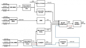
Figure 1: Scheme of the area of raw materials processing

3. The model of thermal tank

Tank has two inlets from which fluid with different temperatures and inflow is flowing to initial volume of certain initial temperature of fluid. Cylindral tank, which has constant diameter, is considered. In tank besides heat transfer between inflow and fluid are also heat transfer between interfaces: fluid-wall of tank, wall of tank-environment. The wall has certain heat capacity, coefficient of thermal conductivity, thickness and density.

Water with density, heat capacity, heat transfer coefficient by convection. The air, with constant temperature and coefficient of heat transfer by convection, as environment is considered. In our case outflow is equal of inflows sum, what means that volume of fluid in tank is constant. Transient characteristics of fluid in tank temperature as well as temperature of environments fluid-wall, wall-air are monitored [4], [1].

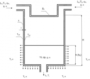
Figure 2: The model of tank with loses to environment

Change of fluid temparature in tank can be expressed by differential equation (1),which comes from energy balance.

(1)

Heat flow of losses is described by follows equation.

(2)

(3)

where: S_P – contact area between wall of tank and fluid [m²]. Changes of temperatures of interfaces fluid – wall and wall – environment are presented in equations 4 and 5.

(4)

(5)

Inputs and parameters for every model are set by table 1.

Table 1: Table of inputs, parameters and values for thermal tank model

Mark	Description	Value	Unit	Type
Iv1	Inflow 1	0,06	m3 .s−1	input
Iv2	Inflow 2	0,08	m3 .s−1	input
T1	Temperature of inflow 1	75	oC	input
T2	Temperature of inflow 2	90	oC	input
Iv	Outflow	0,14	m3 .s−1	parameter
cp	Heat capacity of fluid	4180	J.kg−1.oC−1	parameter
	Density of fluid	1000	kg.m−3	parameter
	Heat transfer coefficient of fluid	2000	W.m−2 .oC−1	parameter
h0	Initial height of fluid	8	m	parameter
S1	Surface of bottom	0,3318	m2	parameter
l	thickness of wall	0,012	m	parameter
	Thermal conductivity of wall	55	W.m−1 .oC−1	parameter
	Density of wall	7800	kg.m−3	parameter
cp	Heat capacity of wall	470	J.kg−1.oC−1	parameter
	Heat transfer coefficient of air	60	W.m−2.oC−1	parameter
T0	Initial temperature of fuid in tank	30	oC	parameter
Tp	Temperature of environment (air)	30	oC	parameter
Tst10	Initial temperature of interface fluid-wall	30	oC	parameter
Tst20	Initial temperature of interface wall-air	30	oC	parameter

4. Implementation of mathematical model

MATLAB Simulink is considered as a strong tool for creation of simulation models in general. It gives several options how to develop simulation models in area processing of raw materials or in other area. Three approaches to create models are introduced and compared in article. The first approach is model created in form of m-function in MATLAB, where differential equations, equations solving method, inputs and parameters are set directly by entering commands in function. Result of the second and third modeling method are independent simulinks blocks. Difference between blocks is in implementation of calculation part of mathematical model.

4.1 Modelling based on m-function creation

Definition of the function:

function Model1

Contents of function model1

• Clearing memory and desktop in MATLAB
• Inputs and parameters definition
• Initial conditions for simulation and solver
• Call the solver for ODE in Temperature ODE
• ODE of the tank model – derived from energy balance

Clearing memory and desktop in MATLAB

Orders from this part close all the open figure windows and clear variables and functions from memory.

clear all;
close all;
clc;

Inputs and parameters definition

Inputs and parameters was set by table 1 to a structure p.

% m^3/s
p.Iv1=0.06; p.Iv2=0.08; p.Iv=p.Iv1+p.Iv2;
% C
p.T1=75; p.T2=90; p.To=30; p.T0=30;
% Wm^-2*C^-1
p.alfa=2000; p.alfa_envi=60;
% W*m^-1*C^-1
p.lambda=55;
% m
p.h=8; p.l=0.012;
% m^2
p.S1=0.3318; p.Sp=2*sqrt(pi*p.S1)*p.h+p.S1;
% kJ*kg^-1*C^-1
p.cpst=470; p.cp=4180;
% kg/m^3
p.rost=7800; p.ro=1000;

Initial conditions for simulation and solver

In first, second and third line are defined initial condition of temperature of fluid in tank and temperatures among interfaces fluid-wall-environment.Fourth line contain simulation time set- ting. Relative tolerance for ODE solver are set in last line.

T0=p.T0; Tst10=p.T0; Tst20=p.To; tspan_1=[0 500]; options=odeset(’RelTol’,1e-4);

Call the solver for ODE in Temperature ODE

It is called solver ode15s for function TemperatureODE. Inputs to solver are differential equa- tion from function TemperatureODE, length of simulation, initial conditions, relative tolerance setted as it showned in previous subsection and inputs structure p.

[t,T]=ode15s(@TemperatureODE,tspan_1,[T0 Tst10 Tst20],options,p);

ODE of the tank model – derived from energy balance

In last part of function Model1 is function TemperatureODE where is differential equation written by mathematical model from section 3. Inputs to function are time of simulation, temperatures and structure p.

function dTdt=TemperatureODE(t,T,p)

4.2 Modelling by simulink blocks

This models approach is also described in [4].

Contents of model2

• Inputs and parameters definition
• Solver setting
• Calculation part

Inputs and parameters definition

Result of modelling approach of model 2 is independent block. Inputs are lead to blok by means of simulink bloks Constant and parameters are imported to the model throught the special form which is showned on figure 3.

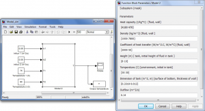
Figure 3: Block of model 2 with inputs and parameters

Solver setting

Initial conditions are set in calculation part of model. Setting of solver and time of simulation are shown in figure 4.

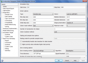
Figure 4: Solver and simulation time setting

Calculation part

Calculation part consist from system of Smulink predefined blocks which represent mathematical model of tank. Initial condition are set in blocks T , T_st1, T_st2 which are pictured on figure 5 [1]

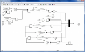
Figure 5: Calculation part of model 2.

4.3 Modelling based on s-function creation

Contents of model3

• Inputs and parameters definition
• Solver setting
• S-function model3

Inputs and parameters definition

Result of modelling approach of Model3 is independent blok. Inputs and parameters are led by the same way as in Model2 what is drawn on figure 3.

Solver setting

Solver seting for Model3 is identical with Model2 seting as is possible to see on figure 4.

S-function

Function is defined follows:

function [sys,x0,str,ts,simStateCompliance]= model3(t,x,u,flag,cp,ro,alfa,h,Ti,dim,Iv)

First part of s-function consist from switcher among different functions in dependence on state of simulation step and type of equation in mathematical model.

switch flag,
case 0, [sys,x0,str,ts,simStateCompliance]= mdlInitializeSizes(n,cp,ro,alfa,h,Ti,dim,Iv );
case 1, sys=mdlDerivatives(t,x,u,n,cp,ro,alfa,h,Ti,dim,Iv );
case 2, sys=mdlUpdate(t,x,u,n,cp,ro,alfa,h,Ti,dim,Iv );
case 3, sys=mdlOutputs(t,x,u,n,cp,ro,alfa,h,Ti,dim,Iv );
case {4,9} sys=[];
otherwise
DAStudio.error(’Simulink:blocks:unhandledFlag’, num2str(flag));
function [sys,x0,str,ts,simStateCompliance]= mdlInitializeSizes(n,cp,ro,alfa,h,Ti,dim,Iv)

In function mdlInitializeSizes are determined number of inputs, outputs, continues states and also discreets states in mathematical moddel. sizes = simsizes;

sizes.NumContStates=3;
sizes.NumDiscStates=0;
sizes.NumOutputs=3;
sizes.NumInputs=4;
sizes.DirFeedthrough=0;
sizes.NumSampleTimes=1;

Initial condition of temperature are inducted to valueble x0 from input parameters valuable(figure 3). Initial value for time is set in last line of initialize part of s-function.

sys = simsizes(sizes);
x0(1)=Ti(2); x0(2)=Ti(2); x0(3)=Ti(1);
str = []; ts =[00];
function sys= mdlDerivatives(t,x,u,n,cp,ro,alfa,h,Ti,dim,Iv )

Function mdlDerivatives is considered as calculation part of hole s-function and simulation model. There can be written diferential equation in time. On our case mathematical model is it equation whic represent mathematical model of tank (section 3).

function sys= mdlOutputs(t,x,u,n,cp,ro,alfa,h,Ti,dim,Iv )
sys(1) = x(1); sys(2) = x(2); sys(3) = x(3);

Output tempretures of every time simulation step (x) are associated to output variable (sys).

5. Simulations

Chosen method for solving of differential equations is stiff/NDF(numerical differential formulas) method. Solver is in MATLAB Simulink known as ode15s. Methods are further discussed in [5].Simulation setting is showed on figure (4). Simulation setting for all simulations is the same. Graphical interpretation of simulation result is generated by function Graphic, which is saving result to file jpg [5], [3].

Figure 6: Graphical results of model1 simulation

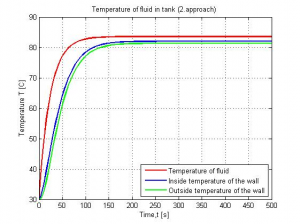
Figure 7: Graphical results of model2 simulation

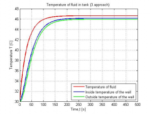
Figure 8: Graphical results of model3 simulation

Figures 6,7,8 comparison is showing that waveforms of temperatures for 1.,2. and 3. simulation model are identical. Identity of temperature waveforms in time for every model is basic condition for approaches comparison.

6. Conclusion

Proposed article describes three ways how to create simulation model of equipment from the area of raw materials processing in MATLAB Simulink by means of balancing elementary processes running inside. Main disadvantage of approach 2(section 4.2) is his low efficiency for more complex models without some of our idealizations. Complexity of differential equations in model 2 can cause less transparent system of simulinks blocks.

In method based on m-function creation (section 4.1) for changing inputs and parameters is necessary to intervene to the source code. Last approach (section 4.3) form viewpoint of user is the most effective because of simple way to change inputs and parameters for simulations. Disadvantage of method 3 (section 4.3) is using only one solving method for every equation in model in contrast to model 1 where is possible to use more than one solver methods. Application of individual modeling methods is influenced by different factors like ability of programmer, complexity of mathematical model and assumed occupancy of model. [4]

Acknowledgement

This work was partially supported by grant VEGA 1/0365/08, 1/0404/08 and 1/4194/06 from the Slovak Grant Agency for Science, and by grant APVV-0040-07 and APVV-20-061905

References

1. M.Fikar J. Mikles. Modelling, identifacation and control of processes. STU Bratislava, Bratislava,SVK, 1999.
2. L.Dorcak J.Terpak. Processes of transformation. Technical univerzity Kosice, Kosice, first edition, 2001.
3. P. Karban. Calculation and simulations in programmes Matlab and Simulink. Computer press, a.s, Brno, CZ, 2005.
4. P. Noskievic. Modelling and identifikation of system. Montanex, Ostrava, CZ, third edition, 1999.
5. J.P. Denier S.R. Otto. An introduction to programming and numerical methods in MATLAB. Springer, London, U.K, 2005.

---

Coauthor of this paper is J. Terpák, B.E.R.G. Faculty, Institute of Control and Informatization of Production Processes, Technical University of Kosice, Slovak Republic