Hybrid predictive controller based on Fuzzy-Neuro model

02. August, 2010, Autor článku: Paulusová Jana, Elektrotechnika, Informačné technológie
Ročník 3, číslo 8 Pridať príspevok

In this paper a hybrid fuzzy-neuro model based predictive control (HFNMBPC) is addressed, proposed and tested. The proposed hybrid fuzzy-neuro convolution model consists of a steady-state fuzzy-neuro model and a gain independent impulse response model. The proposed model is tested in a model based predictive control scheme of the concentration control in the chemical reactor, manipulating its flow rate. The paper deals with theoretical and practical methodology, offering approach for intelligent fuzzy-neuro robust control design and its successful application.

1 Introduction

Predictive control has become popular over the past twenty years as a powerful tool in feedback control for solving many problems for which other control approaches have been proved to be ineffective. Predictive control is a control strategy that is based on the prediction of the plant output over the extended horizon in the future, which enables the controller to predict future changes of the measurement signal and to base control actions on the prediction.

The proposed hybrid fuzzy-neuro convolution model can be considered as a gain-scheduled convolution model. This paper shows advantages of a combination of static nonlinearity and gain- independent dynamic part.

The steady-state behavior of the process is represented by a fuzzy-neuro model structure, which is based on a linguistic knowledge about the steady- state behavior of the process. The parameters of the rule consequents are identified using input and output data gathered from process.

The dynamic part is represented by an impulse response model.

The proposed hybrid fuzzy-neuro convolution model is applied in model predictive control. The HFNMBPC has been received well in process industry.

The paper is organized as follows. First, design of the hybrid fuzzy-neuro convolution model is briefly introduced in Section 2. Then, the fuzzy-neuro model based predictive controller is discussed in Section 3. The reliability and effectiveness of the presented method is shown on application in Section 4 – control of the concentration control in the chemical reactor by manipulating its inlet flow rate. Summary and conclusions are given in Section 5.

2 The Hybrid Fuzzy-Neuro Convolution Model (HFNCM)

The output of the model can be formulated as (Abonyi, et al. 2000)

$y_m (k +1) =$
$\displaystyle = y_s + K (u_s, x_2, \dots ,x_n).\sum ^{N} _{i=1} g_i (u(k-i+1)-u_s)$	(1)

where $y_s + K (u_s,x_2, \dots, x_n)$ is steady-state part, which is described by fuzzy-neuro model (ANFIS) and $\displaystyle \sum^{N} _{i=1} g_i (x_2, \dots , x_n).(u (k - i +1) - u_s)$ is dynamic part of the model (the impulse response model). The gain independent impulse response model is $g_i (x_2, \dots , x_n)$ , the previous input values are $u (k-i-1)$ over N horizon, K is steady-state gain, $u_s$ and $y_s$ are steady -state input and output, $x_2, \dots, x_n$ are other operating parameters having effects on the steady-state output.

The convolution is multiplied by steady-state gain

$K = \frac{\partial f (u_s, x_2, \dots, x_n)}{\partial u_s}$

(2)

2.1 The steady-state part of HFNCM

The steady state part is described by fuzzy-neuro model. A nonlinear discrete system can be expressed by fuzzy-neuro model (ANFIS) with n rules. The i-th rule of the model is described as follows (Paulusová, et al. 2008):

$R^i: if \quad x_1 \quad is \quad A_{1,i} \quad and \dots and \quad x_n \quad is \quad A_{n,i} \quad then \quad y_s = d_i$

(3)

wher $n$ is the number of inputs, $x=[x_1, \dots, x_n]^T$ is a vector of inputs of the model, $A_{j,i} (x_j)$ is the $i=1,2, \dots, M_j$ -th antecedent fuzzy set referring to the j-th input, where $M_j$ is the number of the fuzzy set on the j-th input domain.

The first element of the input vector is the steady- state input $x_i = u_s$ .

The output is computed as weighted average of the individual rules’ consequents

$\displaystyle y_s = \frac{\sum^m _{i=1} \mu_i d_i}{\sum^m _{i=1} \mu_i}$

(4)

where the weights $0 \leq \mu_i \leq 1$ are computed as $\mu_i = \Pi^m _{j=1} A_{ji} (x_j)$ , where $\Pi$ is fuzzy operator, usually been applied as the min or the product operator and m is number of rules.

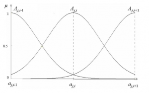
In our research we examined various types of membership functions. In this paper Gaussian membership functions were described in detail.

Gaussian membership functions were employed for each fuzzy linguistic value as shown in Figure 1.

The membership functions are defined as follows:

$\displaystyle A_{j,i-1} (x_j) = e^{- \frac{(x_j - a_{j,i-1})^2}{2 \delta_{j,i-1}^2}}$
$\displaystyle A_{j,i} (x_j) = e^{- \frac{(x_j - a_{j,i})^2}{2 \delta_{j,i}^2}}$	(5)
$\displaystyle A_{j,i+1} (x_j) = e^{- \frac{(x_j - a_{j,i+1})^2}{2 \delta_{j,i+1}^2}}$

where $a_{j,i-1}$ , $a_{j,i}$ , $a_{j,i+1}$ are the centre, $\delta_{j,i-1}$ , $\delta_{j,i}$ , $\delta_{j,i+1}$ dhe width of the fuzzy sets and $x_j \in \quad <a_{j,m_j-1}, a_{j,m_j+1}>$ .

Figure 1 Membership function used for the fuzzy model

The gain of the steady-state fuzzy model can be computed as

$\displaystyle K_j = \frac{\partial y_s}{\partial u_s} =$
$\displaystyle = \sum^{m_j +1} _{i=m_j} \Bigg [ \Bigg ( \frac{\Gamma _{i-1} (u_s)}{a_{1,i} - a_{1,i-1}} - \frac{\Gamma_i (u_s)}{a_{1,i+1} - a_{1,i}} \Bigg ) \Pi ^n _{j=2} A_{j,i} (x_j) d_i \Bigg ]$
$K = \sum ^n _{j=1} K_j$	(6)

where

$\Gamma_i = 1 \quad if \quad u_s \in <a_{1,i}, a_{1,i+1}>$
$\Gamma_i = 0 \quad if \quad u_s \notin <a_{1,i}, a_{1,i+1}>$

2.2 Dynamic part of the HFNCM

The dynamic state part is described by the impulse response model (IRM). Parameters of the discrete IRM $g_i (i = 0, \dots, N)$ where N is the model horizon) can be easily calculated from the input-output data ( $u_i$ and $y_i$ ) of the process.

$\displaystyle y(k) = \sum ^{k} _{i=0} g_i u(k-i)$

(7)

In matrix form

$\displaystyle \left [ \begin{matrix} y_0\\ y_1 \\ \vdots \\ y_N \end{matrix} \right ] = \left [ \begin{matrix} u_0&0&\cdots&0&\cdots \\ u_1&u_0&\cdots&0&\cdots \\ \vdots&\vdots&&&\vdots \\ u_N&u_{N-1}&\cdots&{u_0}&\cdots \end{matrix} \right ] \left [ \begin{matrix} g_0\\ g_1 \\ \vdots \\ g_N \end{matrix} \right ]$

The parameters are given as follows

$\displaystyle g = (U^T U)^{-1}U^{T} y$

(8)

3 Hybrid Fuzzy-Neuro Model Based Predictive Controller

The nonlinear HFNCM can be easily applied in model based predictive control scheme.

In most cases, the difference between system outputs and reference trajectory is used in combination with a cost function on the control effort. A general objective function is the following quadratic form (Paulusová, et al. 2005)

$\displaystyle J = \sum ^p _{i =1} [\hat{y}(k+i\|k) - r(k+i)]^2 \Gamma_y +$
$\displaystyle + \sum^{m} _{i=1}(\Delta u (k+i-1))^2 \Gamma u$	(9)

Here, r is desired set point, $\Gamma_u (\Gamma_u = \gamma K^2)$ and $\Gamma _y$ are weight parameters, determining relative importance of different terms in the cost function, $u$ and $\Delta_u$ are the control signal and its increment, respectively. Parameter p represents length of the prediction horizon, m is the length of the control horizon. Output predicted by the nonlinear fuzzy model is $\hat{y}(k)$ .

$\displaystyle \hat{y}(k) = K \sum ^{\infty} _{i=1} s_i \Delta u (k -i)$

(10)

where $\displaystyle s_i = \sum ^i _{j=1} g_j$ are the step response coefficients and the change on the control variable is $\Delta u (k) = u (k) - u (k - 1)$ .

Model predictions along the prediction horizon p are

$\displaystyle \hat{y}(k +j | k) = K \sum ^{\infty} _{i=1} s_i \Delta u (k +j -i) + e(k +j |k)$

(11)

Disturbances are considered to be constant between sample instants

$\displaystyle e(k +j | k) = y (k | k) - K \sum ^{\infty} _{i=1} s_i \Delta u (k +j -i)$

(12)

where $y (k | k)$ represents the measured value of the process output at time k.

$\displaystyle \hat{y} (k + j |k) = K \sum ^{N} _{i=1} s_i \Delta u (k +j -i) + f (k +j |k)$

(13)

where

$\displaystyle f(k + j | k) = y (k | k) + K \sum ^N _{i=1} (s_{k+1} - s_i) \Delta u (k =i)$

(14)

Prediction of the process output along the length of the prediction horizon, can be written compactly using matrix notation

$\displaystyle \hat{y} (k) = K S \Delta u (k) + f(k)$

(15)

Matrix S is called the system’s dynamic matrix (16) (Morari, et al. 1989).

$\displaystyle S = \left [ \begin{matrix} s_1&0&\cdots&0 \\ s_2&s_1&\cdots&0 \\ \vdots & \vdots & \ddots & \vdots \\ s_m & s_{m-1} & \cdots & s_1 \\ \vdots & \vdots & \ddots & \vdots \\ s_p & s_{p-1}& \cdots & s_{p-m+1} \end{matrix} \right ] _{p \times m}$

(16)

By minimizing its objective function (9) the optimal solution is then given

$\displaystyle \Delta u (k) = \frac{1}{K} (S^T \Gamma_y S + \gamma I)^{-1} S^T \Gamma_y e(k)$

(17)

In many control applications the desired performance cannot be expressed solely as a trajectory following problem. Many practical requirements are more naturally expressed as constraints on process variables such as manipulated variable constraints, manipulated variable rate constraints or output variable constraints. The solution calls into existence of quadratic programming solution of the control problem.

3.1 Algorithm for the HFCM based control

The algorithm has the following steps (Abonyi, et al, 1999):

Calculation impulse response model $g_i$ from (8),
Calculation of $u_s$ from $y_s=y(k)$ , considering the inversion of the fuzzy-neuro model,
Calculation of the value of the steady-state gain K by (6),
Calculation of S by (16) and e by (12),
Calculation of the controller output from the first element of the calculated $\Delta u$ vector generated from (17).

4 Case Study and Simulation Results

4.1 Case study

The application considered involves an isothermal reactor in which the Van Vusse reaction kinetic scheme is carried out. In the following analysis, A is the educt, B the desired product, C and D are unwanted byproducts (Paulusová, et al. 2006).

$\displaystyle A \xrightarrow{\rm k_1} B \xrightarrow{\rm k_2} C$
$\displaystyle 2A \xrightarrow{\rm k_3} D$	(18)

From a design perspective the objective is to make $k_2$ and $k_3$ small in comparison to $k_1$ by appropriate choice of catalyst and reaction conditions. The concentration of B in the product may be controlled by the manipulating the inlet flow rate and/or the reaction temperature.

The educt flow contains only cyclopentadiene in low concentration, $C_{Af}$ . Assuming constant density and an ideal residence time distribution within the reactor, the mass balance equations for the relevant concentrations of cyclopentadiene and of the desired product cyclopentanol, $C_A$ and $C_B$ , are as follows:

$\displaystyle \dot{C}_A = - k_1 C_A - k_3 C_A^2 + \frac{F}{V} (C_{Af} - C_A)$
$\displaystyle \dot{C}_B = k_1 C_A - k_2 C_B - \frac{F}{V} C_b$	(19)
$\displaystyle y =C_B$

This example has been considered by a number of researchers as a benchmark problem for evaluating nonlinear process control algorithm.

By normalizing the process variables around the following operating point and substituting the values for the physical constants, the process model becomes:

$\displaystyle \dot{x}_1(t) = -50 x_1 (t) - 10 x_1^2 (t) + u(10 - x_1 (t))$
$\displaystyle \dot{x}_2 = 50 x_1 (t) - 100 x_2 + u(-x_2 (t))$	(20)
$\displaystyle y (t) = x_2 (t)$

where the deviation variable for the concentration of component A is denoted by $x_1$ , the concentration of component B by $x_2$ , and the inlet flow rate by $u$ .

The simulation scheme of this process is in Figure 2.

Figure 2 Simulation scheme of the nonlinear process described by (20)

4.2 Simulation results

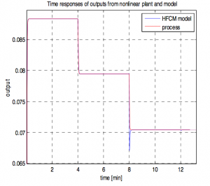
The comparison of HFNCM with nonlinear plant is shown in Figure 3. Time responses of the controlled and reference variables under HFNMBPC are shown in Figure 4.

Figure 3 Time responses of output from the nonlinear plant and the HFNCM model

Figure 4 Time responses of the controlled and reference variables under HFNMBPC ($latex m = 5, \, p = 10, \, \Gamma_y = K, \, \Gamma_u = \gamma K^2, \gamma = 1)

5 Conclusions

The HFMBPC uses the advantage of fuzzy systems in the representation of the steady-state behavior of the system. Other advantage is that it tries to combine knowledge about the system in form of apriori knowledge and measured data in the identification of a control relevant model.

Simulation example illustrates the potential offered by the HFNCMBPC.

Acknowledgements

This paper has been supported by the Slovak Scientific Grant Agency, Grant No. 1/0544/09.

6 References

ABONYI, J.; BÓDIZS, Á., NAGY, L., SZEIFERT, F. (2000). Hybrid fuzzy convolution model and its application in predictive control. Chemical Engineering Research and Design 78 (2000), pp. 597-604.
ABONYI, J.; NAGY, L., SZEIFERT, F. (1999). Fuzzy Model Based Predictive Control by Instantaneous Linearisation. Fuzzy Sets and Systems, 1999.
ABONYI, J.; NAGY, L., SZEIFERT, F. (1999). Adaptive Fuzzy Inference System and its Application in Modelling and Model Based Control, Chem. Eng. Res. Des, 77, A, 281-290, 1999.
MORARI, M.; LEE, J.H.; GARCIA, C.E. (1989). Model Predictive Control. Automatica, vol. 25, no. 3, pp. 335-348, 1989.
PAULUSOVÁ, J.; KOZÁK, Š. (2005). Predictive Fuzzy Control Application. EUROCON 2005- The international Conference on “Computer as a Tool”, Belgrade, Serbia and Montenegro: 21- 24 November, s. 241
PAULUSOVÁ, J.; KOZÁK, Š. (2006). Robust Predictive Fuzzy Control. In.: 7th Portuguese Conference on Automatic Control, CONTROLO’ 2006, Lisbon, Portugal: 11-13 September 2006, MA-7-1. ISBN.
PAULUSOVÁ, J.; KOZÁK, Š.; DÚBRAVSKÁ, M. 2008. Hybrid Predictive Controller based on Fuzzy Model. In: International Slovak Society for Cybernetics and Informatics, Ždiar, Slovak Republic: 10-14 February 2008, pdf 46. ISBN.

Coauthor of this paper is M. Dúbravska, Institute of Control and Industrial Informatics, Faculty of Electrical Engineering and Information Technology, Slovak University of Technology, Ilkovičova 3, 812 19 Bratislava, Slovak Republic

O časopise

Meta

RSS

Hybrid predictive controller based on Fuzzy-Neuro model

Napísať príspevok

Rubriky

Burza práce

Štúdijné materiály

Archív