Control of non-linear processes is a challenging task. One of the ways of control processes like this, is control using neural network, where neural network represents intelligent controller. In this paper, there is proposed a methodology of neural controller design using genetic algorithms. This method allows to find optimal adjustment of neural network weights so that high performance is attained. The proposed control method is verified in Matlab-Simulink on example of isothermal reactor, which represents a real non-linear process.

1 INTRODUCTION

For control of some classes of non-linear dynamic systems with advantage neural controllers (NC) are used. The neural network can be applied as a direct controller. It can emulate expert or another type of controller, it can be direct inverse controller, neuro-predictive controller or optimised by genetic algorithms (GA). This article deals with neural controllers optimised by genetic algorithms. On the Fig. 1, there is depicted the control system with NC optimised by GA (Sekaj, 2003).

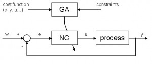
Fig. 1 Block scheme of control system with NC optimised by GA

2 PRELIMINARIES AND PROBLEM FORMULATION

2.1 Neural Controller

Neural controller can be represented by multi layer perceptron (MLP) with one hidden layer. This type of neural network is able to approximate any type of function. Scheme of neural controller is shown on the Fig. 2.

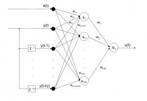
Fig. 2 Scheme of neural controller

Inputs to the neural network are control error e(t), controlled output y(t) and past values of controlled output y(t-i), where i = 1,…,ny and ny is number of past values of controlled output. Output from neural network is control action u(t).

Weights between input and hidden layer are variables w_ij, where i means neuron in input layer (i = 1,.., 2+ny) and j neuron in hidden layer (j = 1,.. HN, HN – number of hidden neurons), which are connected. Weights between hidden and output layer are variables w_k, where k means neuron in hidden layer (k = 1,.., HN), which is connected with single output neuron. Variables b_1k (k = 1,…, HN) are biases in hidden layer and b₂ bias in output layer. (Demuth, 2003; Jadlovská, 2003)

2.2 Genetic Algorithms

Genetic algorithm (GA) is a powerful stochastic-based search/optimisation approach, which mimics the evolution in the nature. It is described in e.g. (Goldberg, 1989; Man, et al., 2001; Michalewicz, 1996; Sekaj, 2005) and others. A general scheme of a GA can be described by following steps (Fig.3):

1. Initialisation of the population of chromosomes (set of randomly generated chromosomes).
2. Evaluation of the cost function (fitness) for all chromosomes.
3. Selection of parent chromosomes.
4. Crossover and mutation of the parents children.
5. Completion of the new population from the new children and selected members of the old population. Jump to the step 2.

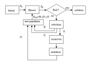
Fig. 3 Block scheme of genetic algorithm

Genetic algorithms fall into the optimisation techniques, which are able to find global optimum of the function. In this case, optimal parameters of neural network (weights and biases) are looking for and optimised function is the cost function:

,

(1)

where the minimum is searching. N represents number of samples in simulation of control, e is control error, r reference variable and y is controlled output. Chromosomes in this case are represented by neural network weights and biases.

After the initialization of the population, fitness of all the chromosomes from population is evaluated. Fitness is represented by cost function (1) or by modified cost function, which can be penalized for example by derivation of process output y, or by measure or derivation of control action u. For evaluation of fitness, simulations of control system are performed for some different step changes in reference variable r.

The algorithm stops, when the specified number of generation is performed and the result is the neural network, which has attained the minimum of fitness.

3 CASE STUDY: ISOTHERMAL REACTOR

3.1 Controlled System

The mathematic model of isothermal reactor is described by differential equations:

,

(2)

,

(3)

Values of reactor parameters:

k₁ = 50 h^-1
k₂ = 100 h^-1
k₃ = 10 mol^-1.l.h^-1
C_af = 10 mol.l^-1
V = 1 l

Input to the system is cubic flow F [l.h^-1] and output from the system is concentration of subject B C_b [mol.l^-1].

There is a model process scheme in Matlab-Simulink in Fig.4.

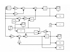
Fig. 4 Model process scheme of isothermal reactor in Matlab-Simulink

Fig. 5 shows transfer characteristic curve of isothermal reactor. The process is highly non-linear with static non-linearity.

Fig. 5 Transfer characteristic curve of isothermal reactor

On the Fig. 6, there are depicted time responses of process output y to different step changes in process input u. Step changes were performed from start input u_s = 0 [l.h^-1] to final inputs u_f: 2.9942, 7.2995, 13.8062, 25.0000 and 70.3626 [l.h^-1].

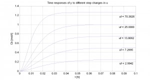
Fig. 6 Time responses of process output y to different step changes in process input u

3.2 Genetic Algorithm

There was proposed genetic algorithm for optimisation of neural controller. It was created for linear system with these functions in Matlab:


Sigma1 = (rangeH-rangeL)/20;
Sigma_a=[Sigma1*ones(1,(4+numdy)*SN+1)];

Sigma2 = (rangeH-rangeL)/200;
Sigma_b=[Sigma2*ones(1,(4+numdy)*SN+1)];

Sigma3 = (rangeH-rangeL)/2000;
Sigma_c=[Sigma3*ones(1,(4+numdy)*SN+1)];

Sigma4 = (rangeH-rangeL)/20000;
Sigma_d=[Sigma4*ones(1,(4+numdy)*SN+1)];

Best=selbest(Pop,Fit,[1,1]);
Old1=[selrand(Pop,Fit,5)];
Old2=genrpop(5,Space);

Work1_a=[selbest(Pop,Fit,[2,2,1])];
Work1_b=[seltourn(Pop,Fit,12)];
Work1 = [Work1_a;Work1_b];
Work2=[selbest(Pop,Fit,[1])];

Work1=crossov(Work1,4,0);

Work1=mutx(Work1,0.1,Space);
Work1=muta(Work1,0.1,Sigma_a,Space);
Work1=muta(Work1,0.3,Sigma_b,Space);
Work1=muta(Work1,0.5,Sigma_c,Space);
Work1=muta(Work1,0.7,Sigma_d,Space);
Work2=muta(Work2,0.1,Sigma_a,Space);
Work2=muta(Work2,0.3,Sigma_b,Space);
Work2=muta(Work2,0.5,Sigma_c,Space);
Work2=muta(Work2,0.7,Sigma_d,Space);

Pop=[Best;Old1;Old2;Work1;Work2];

3.3 Optimisation of Neural Controller

For control of isothermal reactor, neural controller was proposed. Inputs to the neural network are control error e, controlled output y and numdy past values of controlled output. The neural network has HN neurons in hidden layer. Range of weight and bias values is from rangeL to rangeH and number of generation is numgen.

On the Fig. 7, there are shown time responses of controlled output y and control action u to different step changes in reference variable r from starting reference value rs = 0 mol.l^-1 with following parameters of neural controller and genetic algorithm:

numdy = 7
HN = 25
rangeL = -20
rangeH = 20
numgen = 200

For fitness, the cost function (1) was used. Nearly all of the time responses were settled on reference values, without time response of y to step change to highest value of final reference value r_f = 1.264 mol.l^-1. Overshoots of time responses of controlled output are very large, for step change to r_f = 0.25 mol.l^-1 the overshot is nearly 100%.

Fig. 7 Time responses of controlled output y and control action u to different step changes in reference variable r for first case

On the Fig. 8, there are also shown time responses of controlled output y and control action u to different step changes in reference variable r from starting reference value r_s = 0 mol.l^-1. There were used same parameters and same fitness and cost function as in the previous case. The difference is in the use of limitations in control action u. Low limitation is u_limL = 0 l.h^-1 and high limitation is u_limH = 77 l.h^-1.

Now, steady-state error and also overshoots are smaller and controlled times are shorter than those in the previous case. On the Fig. 9, there is shown best fitness in dependence on generation for this case. The curve is settled in 200^th generation under the fitness equals 200.

Fig. 8 Time responses of controlled output y and control action u to different step changes in reference
variable r for second case

Fig. 9 Best fitness of population in dependence on generation for second case

In the next case, there are used the same adjustments of parameters as in the previous cases and the same limitations of control action u as in the second case. The difference is in the fitness. It is modified cost function with penalization by derivation of process output y:

,

(4)

N represents number of samples, e is control error and dy is derivation of process output. This penalization should limit oscillating in controlled output y. The time responses are depicted on the Fig. 10.
The dynamics is different from the previous case. Overshoots are smaller, but there is steady-state error too, for step change to r_f = 0.25 mol.l^-1.

Fig. 10 Time responses of controlled output y and control action u to different step changes in reference variable r for third case

On the Fig. 11 and Fig. 12, there are shown best fitness (Fig. 11) and appropriate value of cost function (Fig. 12) in dependence on generation. The curve of the best fitness is settled in 160^th generation. Final value of cost function is smaller than 200, like in the previous case. There isn’t better solution between this and the previous case.

Fig. 11 Best fitness of population in dependence on generation for third case

Fig. 12 Cost function in dependence on generation for third case

4 CONCLUSION

Genetic algorithms are an efficient mean for neural controller optimisation however, it is a challenging task. It is necessary to choose parameters of genetic algorithm properly and also parameters of neural network. The problem can be also choosing of right fitness.

The goal of the presented project is to proposed neural controller using genetic algorithms for non-linear process. The proposed neural networks for isothermal reactor control are useful, but there is a problem with a steady-state error. It can be eliminated using integration of control error as the input to the neural controller.

Neural controller is able to provide for high performance for non-linear systems.

REFERENCES

1. Demuth, H. and M. Beale (2003). Neural Network Toolbox, For use with Matlab, User’s guide.
2. Goldberg, D.E. (1989). Genetic Algorithms in Search, Optimisation and Machine Learning. Addisson-Wesley.
3. Jadlovská, A. (2003). Modelovanie a riadenie dynamických procesov s využitím neurónových sietí. Informatech, Košice.
4. Man, K.F., K.S. Tang and S. Kwong (2001). Genetic Algorithms, Concepts and Deign. Springer.
5. Michalewicz, Z. (1996). Genetic Algorithms + Data Structures = Evolutionary Programs. Springer.
6. Sekaj, I. (2003). Genetic Algorithm Based Controller Design. In: 2nd IFAC conference Control System Design’03. Bratislava.
7. Sekaj, I. (2005). Evolučné výpočty a ich využitie v praxi. Iris, Bratislava.

---

Co-author of this paper is Slavomír Kajan, Slovak University of Technology, Faculty of Electrical Engineering and Information Technology, Ilkovičova 3, 812 19 Bratislava.