Direct Model Reference Adaptive Control of Small Laboratory DC Motor

10. Január, 2011, Autor článku: Tárník Marián, Elektrotechnika, Študentské práce
Ročník 4, číslo 1 Pridať príspevok

Plants can be modeled with different types of mathematical models. A plant model which is suitable for control design may be developed by using physical laws or by processing the plant I/O data by using appropriate identification method. Usually a simple linear model leads to a simple controller. However, more accurate or exact description of the plant is nonlinear and/or time varying and this description usually can not be used for control design.

In many cases, for a given operating point, the complex plant dynamics can be ap- proximated by a linear time invariant (LTI) model with the given structure and constant parameters. When the operating point changes, then the parameters has to be changed for the appropriate approximation of plant dynamics while structure of the model usually remains unchanged. Therefore, a simple controller designed for the given operating point is unable to achieve the desired control performance in the different operating points.

In the Adaptive Control the controller structure consists of a feedback loop and a controller with adjustable gains. The gains of controller are then changed so that the control performance requirements are met for different operating points.

Purpose of this work is to demonstrate the design of the Model Reference Adaptive Control based on MRC problem for a general class of LTI SISO plants by using it to control a real laboratory plant. Detailed analysis of the presented control schemes and procedures can be found in Ioannou(1996). In this paper the controlled plant is a small laboratory DC motor with the auxiliary electronics which provides the connection to computer and allows to adjust the overall system dynamics.

In this article the electronic adjustment of the system dynamics is set on certain value and remains unchanged. Pos- sible changes in the dynamics are due to changes in plant operating point. Input of the plant is the supply voltage from the range ⟨0, 10⟩ [V]. Output is the angular frequency. Information about angular frequency is obtained using the tachodynamo. Therefore output is in volts from the range ⟨0,10⟩ [V]. For more detail see Kajan(2007).

2. The plant model

Consider the two operating points given by plant output values: y_OP1 = 3V and y_OP2 = 5V . Values of the plant input for this operating points can be found experimentaly. Then the data for identification are obtained by using an appropriate input step signal arround the found input values of the plant. It is assumed that in the range y_OP ± 0.4V the plant dynamics does not change. The result of the plant identification in two operating points by using AutoregRessive model with eXogenous variable (ARX) method are two transfer functions:

$G_{OP_1} = 0.1659 \frac{s + 22}{ s^2 + 3.1423 s + 2.6539}$

(1)

$G_{OP_2} = 0.1669 \frac{s + 20.7618}{s^2 + 2.3422s + 2.7293}$

(2)

This result clearly show that the system parameters vary with changes in operating point.

3. The MRC problem

The MRC objective is to determine the plant input u_p so that the plant output y_p tracks the reference model output ym for given reference input r(t). Consider the SISO LTI plant described by the transfer function

$G_p(s)= \frac{y_p}{u_p} = k_p \frac{Z_p(s)}{R_p(s)}$

(3)

where k_p is the constant with known sign, R_p(s) is the monic polynomial and Z_p(s) is a monic Hurwitz polynomial. The general assumption is that an upper bound of the degree of R_p(s) and the relative degree are known, but for simplicity let us assume in the next section that the degree n of Z_p(s) and the degree m of Rp(s) are known. The relative degree is n* = n − m.

The reference model describes the desired characteristics of the plant and it is selected by the designer. Consider the reference model in the transfer function form

$W_m(s) = \frac{y_m}{r} = k_m \frac{Z_m(s)}{R_m(s)}$

(4)

where k_m is the constant and Z_m(s), R_m(s) are monic polynomials. Transfer function W_m(s) is designed to be strictly positive real (SPR).

Consider the control law in the form

$u_p = {\boldsymbol{\mathsf{\Theta}}_1^\star}^{\mathsf{T}} \frac{\alpha(s)}{\Lambda(s)} u_p + {\boldsymbol{\mathsf{\Theta}}_2^\star}^{\mathsf{T}} \frac{\alpha(s)}{\Lambda(s)} y_p + \mathsf{\Theta}_3^\star y_p + \mathsf{\Theta}_4^\star r$

(5)

where $\alpha(s) = \begin{bmatrix} s^{n-2}, \ldots,s, 1 \end{bmatrix}^{\mathsf{T}}$ if $n\geq 2$ , otherwise $\alpha(s) = 0$ , and ${\boldsymbol{\mathsf{\Theta}}_1^\star}, {\boldsymbol{\mathsf{\Theta}}_2^\star} \in \mathcal{R}^{n-1};$ $\mathsf{\Theta}_3^\star, \mathsf{\Theta}_4^\star \in \mathcal{R}^1$ are constant prarameters to be designed. $\Lambda(s)$ is an arbitrary monic Hurwitz polynomial of degree n-1 with Z_m(s) as an factor

$\Lambda(s) = \Lambda_0(s) Z_m(s)$

(6)

In Ioannou(1996) is shown that there exist a parameters ${\boldsymbol{\mathsf{\Theta}}_1^\star}, {\boldsymbol{\mathsf{\Theta}}_2^\star}, \mathsf{\Theta}_3^\star, \mathsf{\Theta}_4^\star$ for which the closed loop transfer function, consisting (3) and (5), equals to the reference model transfer function (4).

3.1 Particular case

Instead of considering the general form of the control law (5) and the general plant model, MRC problem for the plant model in the form

$y_p = k_p \frac{s + b_0}{ s^2 + a_1 s + a_0} \, u_p$

(7)

is solved in this section. In (7) a_i,b_i are constant. Notice that the transfer function (7) has the same form as the plant model (1) and (2). The model reference is chosen to have the same relative degree as the plant

$y_m = W_m(s)r = k_m \frac{s + b_{m0}}{ s^2 + a_{m1} s + a_{m0}} r$

(8)

In this case the control law has the form

$u_p = \mathsf{\Theta}_1^\star \frac{1}{(s + \lambda)} u_p + \mathsf{\Theta}_2^\star \frac{1}{(s + \lambda)} y_p + \mathsf{\Theta}_3^\star y_p + \mathsf{\Theta}_4^\star r$

(9)

where we use $\alpha(s) = 1$ and $\Lambda(s) = (s + \lambda)$ . The control law (9) can be written in the form

$u_p = \frac { \mathsf{\Theta}_2^\star + \mathsf{\Theta}_3^\star (s + \lambda)} { (s + \lambda) - \mathsf{\Theta}_1^\star } y_p + \frac {\mathsf{\Theta}_4^\star (s + \lambda)} {(s + \lambda) - \mathsf{\Theta}_1^\star} r$

(10)

The closed loop transfer function is obtained by substituing (10) to (7), then:

$\frac{y_p}{r} = G_c(s) =\frac { k_p (s + b_0) \mathsf{\Theta}_4^\star (s + \lambda) } { (s^2 + a_1 s + a_0) \left( (s + \lambda) - \mathsf{\Theta}_1^\star \right) - k_p (s + b_0) \left( \mathsf{\Theta}_2^\star + \mathsf{\Theta}_3^\star (s + \lambda) \right) }$

(11)

The matching equation is G_c(s) = W_m(s). Choosing

$\mathsf{\Theta}_4^\star = \frac{k_m}{k_p}$

(12)

$\lambda = b_{m0}$

(13)

the matching equation becomes

$(s^2 + a_1 s + a_0) \left( (s + \lambda) - \mathsf{\Theta}_1^\star \right) - k_p (s + b_0) \left( \mathsf{\Theta}_2^\star + \mathsf{\Theta}_3^\star (s + \lambda) \right)$

$= (s + b_0) ( s^2 + a_{m1} s + a_{m0})$

(14)

which can be expressed in terms of the matrix algebraic equation by equating the coefficients of the powers of s on both sides. Then we have

$\begin{bmatrix} -1 & 0 & -k_p \\ -a_1 & -k_p & -(k_p b_{m0} + k_p b_0) \\ -a_0 & -k_p b_0 & -k_p b_0 b_{m0} \end{bmatrix} \begin{bmatrix} \mathsf{\Theta}_1^\star \\ \mathsf{\Theta}_2^\star \\ \mathsf{\Theta}_3^\star \end{bmatrix}$

$= \begin{bmatrix} a_{m1} + b_0 - b_{m0} - a_1 \\ a_{m0} + b_0 a_{m1} + a_1 b_{m0} - a_0 \\ b_0 a_{m0} - a_0 b_{m0} \end{bmatrix}$

(15)

In the case when the plant parameters are known the control law (9), with parameters (12) and (15), solves the MRC problem. This means that the closed loop transfer function G_c(s) equals to the reference model transfer function W_m(s).

4. State space representation of the closed loop system

The plant (7) can be represented in state space in the form

$\dot{\boldsymbol{\mathsf{x}}} = \boldsymbol{\mathsf{A}} \boldsymbol{\mathsf{x}} + \boldsymbol{\mathsf{b}} u_p$

(16)

$y_p = \boldsymbol{\mathsf{c}}^{\mathsf{T}} \boldsymbol{\mathsf{x}}$

(17)

where $\boldsymbol{\mathsf{x}}$ is state vector of plant and $\boldsymbol{\mathsf{A}}; \boldsymbol{\mathsf{b}}; \boldsymbol{\mathsf{c}}^{\mathsf{T}}$ are constant matrices with appropriate dimensions. The control law (9) can be represented in the state space in the form

$\dot{\nu}_1 = -\lambda \nu_1 + u_p$

(18)

$\dot{\nu}_2 = -\lambda \nu_2 + \boldsymbol{\mathsf{c}}^{\mathsf{T}} \boldsymbol{\mathsf{x}}$

(19)

$u_p = \boldsymbol{\mathsf{\Theta}}^{\mathsf{T}} \boldsymbol{\mathsf{D}} \boldsymbol{\mathsf{X}} + \mathsf{\Theta}_4 r$

(20)

where $\boldsymbol{\mathsf{\Theta}} = \begin{bmatrix} \mathsf{\Theta}_3 & \mathsf{\Theta}_1 & \mathsf{\Theta}_2 \end{bmatrix}^{\mathsf{T}} ; \; \mathsf{\Theta}_4$ are the control law parameters, $\boldsymbol{\mathsf{D}} = \begin{bmatrix} \boldsymbol{\mathsf{c}}^{\mathsf{T}} & 0 & 0 \\ 0 & 1 & 0 \\ 0 & 0 & 1 \end{bmatrix}$ and $\boldsymbol{\mathsf{X}} = \begin{bmatrix} \boldsymbol{\mathsf{x}} \\ \nu_1 \\ \nu_2 \end{bmatrix}$ . In the case of known plant parameters the parameters of control law are known: $\boldsymbol{\mathsf{\Theta}}^\star ; \; \mathsf{\Theta}_4^\star$ . Including of the auxiliary states $\nu_1$ and $\nu_2$ to the plant states space representation leads to following equations

$\dot{\boldsymbol{\mathsf{X}}} = \boldsymbol{\mathsf{A}}_o \boldsymbol{\mathsf{X}} + \boldsymbol{\mathsf{B}}_c u_p$

(21)

$y_p = \boldsymbol{\mathsf{C}}_c^{\mathsf{T}} \boldsymbol{\mathsf{X}}$

(22)

where

$\boldsymbol{\mathsf{A}}_o = \begin{bmatrix} \boldsymbol{\mathsf{A}} & 0 & 0 \\ 0 & -\lambda & 0 \\ \boldsymbol{\mathsf{c}}^{\mathsf{T}} & 0 & -\lambda \end{bmatrix} ;\quad \boldsymbol{\mathsf{B}}_c = \begin{bmatrix} \boldsymbol{\mathsf{b}} \\ 1\\ 0 \end{bmatrix} ;\quad \boldsymbol{\mathsf{C}}_c = \begin{bmatrix} \boldsymbol{\mathsf{c}} \\ 0\\ 0 \end{bmatrix}$

In this paper we refer to equation (21) and (22) as an augmented plant equations. The ideal closed loop transfer function is obtained by substituing the control law with known parameters to the augmented plant equation (21), i.e.,

$\dot{\boldsymbol{\mathsf{X}}} = \boldsymbol{\mathsf{A}}_c \boldsymbol{\mathsf{X}} + \boldsymbol{\mathsf{B}}_c \mathsf{\Theta}_4^\star r$

(23)

$y_p = \boldsymbol{\mathsf{C}}_c^{\mathsf{T}} \boldsymbol{\mathsf{X}}$

(24)

where $\boldsymbol{\mathsf{A}}_c = \boldsymbol{\mathsf{A}}_o + \boldsymbol{\mathsf{B}}_c {\boldsymbol{\mathsf{\Theta}}^\star}^{\mathsf{T}} \boldsymbol{\mathsf{D}}$ , which imlpies that

$G_c(s) = \boldsymbol{\mathsf{C}}_c^{\mathsf{T}} \left( s \boldsymbol{\mathsf{I}} - \boldsymbol{\mathsf{A}}_c \right)^{-1} \boldsymbol{\mathsf{B}}_c \mathsf{\Theta}_4^\star = W_m(s)$

(25)

This also means, that the reference model can be decribed by the nonminimal state space representation in the form

$\dot{\boldsymbol{\mathsf{X}}}_m = \boldsymbol{\mathsf{A}}_c \boldsymbol{\mathsf{X}}_m + \boldsymbol{\mathsf{B}}_c \mathsf{\Theta}_4^\star r$

(26)

$y_m = \boldsymbol{\mathsf{C}}_c^{\mathsf{T}} \boldsymbol{\mathsf{X}}_m$

(27)

5. Direct Adaptive law

Because the parameters of the plant changes with the operating point we assume that they are unknown. Therefore the desired controller parameters $\boldsymbol{\mathsf{\Theta}}^\star, \, \mathsf{\Theta}_4^\star$ cannot be calculated from the matching equation. Thus the unknown control law parameters are replaced by the $\boldsymbol{\mathsf{\Theta}}(t), \, \mathsf{\Theta}_4(t)$ which are the estimates of $\boldsymbol{\mathsf{\Theta}}^\star, \, \mathsf{\Theta}_4^\star$ at time t to be generated by an appropriate adaptive law.

Finding of the adaptive law can be viewed as a on-line identification problem of the unknown constants $\boldsymbol{\mathsf{\Theta}}^\star, \, \mathsf{\Theta}_4^\star$ . The augmented plant (21) can be expressed in terms of $\boldsymbol{\mathsf{\Theta}}^\star, \, \mathsf{\Theta}_4^\star$ by adding and substracting the desired input term $u_p^\star = \boldsymbol{\mathsf{B}}_c {\boldsymbol{\mathsf{\Theta}}^\star}^{\mathsf{T}} \boldsymbol{\mathsf{D}} \boldsymbol{\mathsf{X}} + \boldsymbol{\mathsf{B}}_c \mathsf{\Theta}_4^\star r$ to obtain

$\dot{\boldsymbol{\mathsf{X}}} = \boldsymbol{\mathsf{A}}_c \boldsymbol{\mathsf{X}} + \boldsymbol{\mathsf{B}}_c \mathsf{\Theta}_4^\star r + \boldsymbol{\mathsf{B}}_c \left( u_p - {\boldsymbol{\mathsf{\Theta}}^\star}^{\mathsf{T}} \boldsymbol{\mathsf{D}} \boldsymbol{\mathsf{X}} - \mathsf{\Theta}_4^\star r \right)$

(28)

$y_p = \boldsymbol{\mathsf{C}}_c^{\mathsf{T}} \boldsymbol{\mathsf{X}}$

(29)

which is the parametrization of the plant equation in terms of the ideal controller parameters. Let

$\boldsymbol{\mathsf{e}} = \boldsymbol{\mathsf{X}} - \boldsymbol{\mathsf{X}}_m$

(30)

$e_1 = y_p - y_m$

(31)

then the error equation has the form

$\dot{\boldsymbol{\mathsf{e}}} = \boldsymbol{\mathsf{A}}_c \boldsymbol{\mathsf{e}} + \boldsymbol{\mathsf{B}}_c \left( u_p - {\boldsymbol{\mathsf{\Theta}}^\star}^{\mathsf{T}} \boldsymbol{\mathsf{D}} \boldsymbol{\mathsf{X}} - \mathsf{\Theta}_4^\star r \right)$

(32)

$e_1 = \boldsymbol{\mathsf{C}}_c^{\mathsf{T}} \boldsymbol{\mathsf{e}}$

(33)

$e_1 = W_m(s) \frac{1}{\mathsf{\Theta}_4^\star} \left( u_p - {\boldsymbol{\mathsf{\Theta}}^\star}^{\mathsf{T}} \boldsymbol{\mathsf{D}} \boldsymbol{\mathsf{X}} - \mathsf{\Theta}_4^\star r \right)$

(34)

The estimate $\hat{e}_1$ of $e_1$ based on $\boldsymbol{\mathsf{\Theta}}(t)$ and $\mathsf{\Theta}_4(t)$ is given by

$\hat{e}_1 = W_m(s) l \left( u_p - {\boldsymbol{\mathsf{\Theta}}}^{\mathsf{T}} \boldsymbol{\mathsf{D}} \boldsymbol{\mathsf{X}} - \mathsf{\Theta}_4 r \right)$

(35)

where $l$ is estimate of $1/\mathsf{\Theta}_4^\star$ . Because $u_p = {\boldsymbol{\mathsf{\Theta}}}^{\mathsf{T}} \boldsymbol{\mathsf{D}} \boldsymbol{\mathsf{X}} + \mathsf{\Theta}_4 r$ is considered it follows that $\hat{e}_1 = 0$ . Therefore there is no need to form the error estimation model (35), and the estimation error is simply the tracking error $e_1$ . Substituting for the control law in (32), we obtain the error equation

$\dot{\boldsymbol{\mathsf{e}}} = \boldsymbol{\mathsf{A}}_c \boldsymbol{\mathsf{e}} + \overline{\boldsymbol{\mathsf{B}}}_c \frac{1}{\mathsf{\Theta}_4^\star} \left( {\boldsymbol{\mathsf{\theta}}}^{\mathsf{T}} \boldsymbol{\mathsf{D}} \boldsymbol{\mathsf{X}} + \mathsf{\theta}_4 r \right)$

(36)

$e_1 = \boldsymbol{\mathsf{C}}_c^{\mathsf{T}} \boldsymbol{\mathsf{e}}$

(37)

where $\overline{\boldsymbol{\mathsf{B}}}_c = \boldsymbol{\mathsf{B}}_c \mathsf{\Theta}_4^\star$ , or

${e}_1 = W_m(s) \frac{1}{\mathsf{\Theta}_4^\star} \left( {\boldsymbol{\mathsf{\theta}}}^{\mathsf{T}} \boldsymbol{\mathsf{D}} \boldsymbol{\mathsf{X}} + \mathsf{\theta}_4 r \right)$

(38)

which relates the parameter errors ${\boldsymbol{\mathsf{\theta}}} = {\boldsymbol{\mathsf{\Theta}}} - {\boldsymbol{\mathsf{\Theta}}^\star}$ and $\mathsf{\theta}_4 = \mathsf{\Theta}_4 - \mathsf{\Theta}_4^\star$ with the tracking error $e_1$ through the SPR transfer function. This motivates the use of the SPR-Lyapunov design aproach to ensure asymptotic stability of tracking error $e_1$ . Consider the Lyapunov-like function

$V = \boldsymbol{\mathsf{e}}^{\mathsf{T}} \boldsymbol{\mathsf{P}} \boldsymbol{\mathsf{e}} + \left| \frac{1}{\mathsf{\Theta}_4^\star} \right| {\boldsymbol{\mathsf{\theta}}}^{\mathsf{T}} \boldsymbol{\mathsf{\Gamma}}^{-1} {\boldsymbol{\mathsf{\theta}}} + \left| \frac{1}{\mathsf{\Theta}_4^\star} \right| \gamma^{-1} \mathsf{\theta}_4^2$

(39)

where $\boldsymbol{\mathsf{\Gamma}} = \boldsymbol{\mathsf{\Gamma}} ^{\mathsf{T}} > 0$ , $\gamma > 0$ are the design parameters of adaptive law and $\boldsymbol{\mathsf{P}} = \boldsymbol{\mathsf{P}}^{\mathsf{T}} > 0$ satisfies the algebraic equation implied by Mayer-Kalman-Yakubovich (MKY) lemma: If $W_m(s) = \boldsymbol{\mathsf{C}}_c^{\mathsf{T}} \left( s \boldsymbol{\mathsf{I}} - \boldsymbol{\mathsf{A}}_c \right)^{-1} \overline{\boldsymbol{\mathsf{B}}}_c$ is SPR, then we can write

$\boldsymbol{\mathsf{A}}_c^{\mathsf{T}} \boldsymbol{\mathsf{P}} + \boldsymbol{\mathsf{P}} {\boldsymbol{\mathsf{A}}_c} = - {\boldsymbol{\mathsf{Q}}}$

(40)

$\boldsymbol{\mathsf{P}} {\boldsymbol{\mathsf{B}}_c} = {\boldsymbol{\mathsf{C}}_c}$

(41)

where $\boldsymbol{\mathsf{Q}} = \boldsymbol{\mathsf{Q}}^{\mathsf{T}} > 0$ . The time derivate $\dot{V}$ of $V$ along the trajectory of (36) is given by

$\dot{V} = \boldsymbol{\mathsf{e}}^{\mathsf{T}} \left( - \boldsymbol{\mathsf{Q}} \right) \boldsymbol{\mathsf{e}} + \frac{2}{\mathsf{\Theta}_4^\star} \boldsymbol{\mathsf{e}}^{\mathsf{T}} \boldsymbol{\mathsf{P}} \boldsymbol{\mathsf{B}}_c \boldsymbol{\mathsf{\theta}}^{\mathsf{T}} \boldsymbol{\mathsf{D}} \boldsymbol{\mathsf{X}} + \frac{2}{\mathsf{\Theta}_4^\star} \boldsymbol{\mathsf{e}}^{\mathsf{T}} \boldsymbol{\mathsf{P}} \boldsymbol{\mathsf{B}}_c \mathsf{\theta}_4 r$

$+ \left| \frac{2}{\mathsf{\Theta}_4^\star} \right| \boldsymbol{\mathsf{\theta}}^{\mathsf{T}} \boldsymbol{\mathsf{\Gamma}}^{-1} \dot{\boldsymbol{\mathsf{\theta}}} + \left| \frac{2}{\mathsf{\Theta}_4^\star} \right| \gamma^{-1} \mathsf{\theta}_4 \dot{\mathsf{\theta}}_4$

(42)

The adaptation law results from $\dot{V} \leq 0$ requirement. Choosing

$\dot{\boldsymbol{\mathsf{\theta}}} = -\text{sgn} \left( \frac{1}{\mathsf{\Theta}_4^\star} \right) e_1 \boldsymbol{\mathsf{\Gamma}} \boldsymbol{\mathsf{D}} \boldsymbol{\mathsf{X}}$

(43)

$\dot{\mathsf{\theta}}_4 = -\text{sgn} \left( \frac{1}{\mathsf{\Theta}_4^\star} \right) e_1 \gamma r$

(44)

where
$\boldsymbol{\mathsf{e}}^{\mathsf{T}} \boldsymbol{\mathsf{P}} \boldsymbol{\mathsf{B}}_c = e_1$ and $\frac{1}{\mathsf{\Theta}_4^\star} = \left| \frac{1}{\mathsf{\Theta}_4^\star} \right| \text{sgn} \left( \frac{1}{\mathsf{\Theta}_4^\star} \right)$ is used, leads to

$\dot{V} = \boldsymbol{\mathsf{e}}^{\mathsf{T}} \left( - \boldsymbol{\mathsf{Q}} \right) \boldsymbol{\mathsf{e}} \leq 0$

(45)

Because ideal parameters $\boldsymbol{\mathsf{\Theta}}^\star, \, \mathsf{\Theta}_4^\star$ are considered to be constant (or quasistationary) we have $\dot{\boldsymbol{\mathsf{\theta}}} =\dot{\boldsymbol{\mathsf{\Theta}}}$ and $\dot{\mathsf{\theta}}_4 = \dot{\mathsf{\Theta}}_4$ . Further analysis shows, see Ioannou(1996), that all the signals int the closed-loop system are bounded, and the tracking error goes to zero as $t \to \infty$ .

6. Simulation and experimental results

For simulation the nominal transfer function is used instead of the real plant. The parameters of the nominal transfer function are the average values of identified parameters of the transfer functions (1) and (2). The nominal transfer function is

$G_{n}(s) = 0.1664 \frac{s + 21.3809}{ s^2 + 2.7423 s + 2.6916}$

(46)

The reference model transfer function is considered in the form

$W_m(s) = \frac{s + 3}{ s^2 + 3.5 s + 3}$

(47)

Now, equations (12), (13) and (15) are used to calculate the ideal controller parameter for the nominal case

$\mathsf{\Theta}_4^\star = 6.0096; \quad \boldsymbol{\mathsf{\Theta}}^\star = \begin{bmatrix} -4.5538 & -18.3809 & 11.8080 \end{bmatrix}^{\mathsf{T}}$

These values serves for better estimation of the initial values of control law parameters. Let the initial controller parameters to be close to these values, i.e.,

$\mathsf{\Theta}_{4 init} = 8; \quad \boldsymbol{\mathsf{\Theta}}_{init} = \begin{bmatrix} -4 & -18 & 6 \end{bmatrix}^{\mathsf{T}}$

The reference model is chosen to have slower dynamics as the nominal plant model (46). Reason for this is an effort to avoid the control output to reach its constraints, which allows to the intended demonstration to be lucid.

For the same reason the selected reference signal r contains only low frequencies. The reference signal slowly raise up to the area of operating point 2 (r = 5 ± 0.4V ) where the real plant transfer function is close to (2). Then the value of r slowly moves to the area of operating point 1 (r = 3 ± 0.4V ) and finally it again raise up to the operating point 1. Whole sequence takes 90 seconds.

The process of adaptation is expected in the real experiment because the real plant parameter values changes with operating point. However, in simulation is used a plant whith parameters which does not depend on operating point. Therefore significant process of adaptation is expected only at the begining of simulation experiment.

Choosing of the so called adaptation gains $\boldsymbol{\mathsf{\Gamma}}$ and $\gamma$ has influence on speed and oscillations in adapted parameter convergence. The larger the $\boldsymbol{\mathsf{\Gamma}}$ and $\gamma$ are, the faster the convergence is, but excessive increase in these gains leads to oscillations in the adapted parameter response.

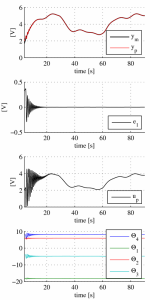
Let choose $\boldsymbol{\mathsf{\Gamma}} = 10 \cdot \boldsymbol{\mathsf{I}}$ and $\gamma = 10$ for first simulation experiment. The result is in the Fig.\ref{First simulation experiment}. There are significant oscilations in the responses caused by excessive value of adaptation gains. Therefore these adaptation gain values are not suitable for real experiment. A good set of the adaptation gain values was found to be

$\boldsymbol{\mathsf{\Gamma}} = \begin{bmatrix} 0.4 & 0 & 0 \\ 0 & 0.1 & 0 \\ 0 & 0 & 0.3 \end{bmatrix} ; \quad \gamma = 0.08$

(48)

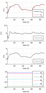
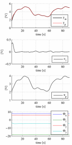
These values has been obtained by using the trail and error method, performing appro- priate number of experiments with the real plant. The result with these adaptation gains is in the Fig.2. Simulation with adaptation gains (48) has been also performed. The result of this simulation is in the Fig.3.

7. Conclusion

This work presents an application of the clasical Model Reference Adaptive Control. First the identification of the controled plant is performed in the two different operating points. The two identified transfer functions differs in the parameter values. It can be considered that the simple controller which is designed to meet the desired control quality in one operating point can not satisfy the quality requirements in the second
operating point.

This can bee seen as a motivation to choose more sophisticated control design. One of the posibilities is Adaptive control. Therefore, the whole MRAC alghoritm for the considered particular case is derived. The matching equation which solves the MRC problem is expressed in the form that allows to immediately compute the controller parameters if the plant and reference model parameters are known.

Figure 1: Result of the first simulation experiment. There are significant oscilations in the responses caused by excessive value of adaptation gains.

Figure 2: Result of experiment with the real plant

Figure 3: Simulation experiment with the same adjustment of control system as in real experiment

The uncommon state space represntation of the control law is used, where matrix D is introduced. This form of control law together with the introduced augmented plant makes derivation of adaptation law similar to case when the state controller is considered. Then it is easyer to see that the derivation procedure is same as in the common simple scalar examples usually described in textbooks (see References).

The use of the SPR-Lyapunov design is shown in detail in this paper. However the further analysis of the obtained results is considered to be out of scope of this demonstration. Finally, the performance of the designed direct MRAC alghoritm is confirmed by simulation experiments and also by experimental results.

References

Åström K.J., Wittenmark B. (1995) Adaptive Cotrol. 2nd edition. Addison-Wesley, ISBN 9780201558661
Butler H. Model Reference Adaptive Control: From theory to practice. Prentice Hall International (UK) Ltd. ISBN 0-13-588286-9
Ioannou P., Sun J. (1996). Robust Adaptive Control. Prentice Hall, Inc, electronic copy at www-rcf.usc.edu/ ioannou/Robust_Adaptive_Control.htm
Ioannou P., Fidan B. (2006) Adaptive Control Tutorial. Society for Industrial and Applied Mathematics, USA.
Kajan S., Hypiusová M. (2007). LABREG Software for Identification and Con- trol of Real Processes in Matlab. Proceedings of Conference Technical Computing Prague 2007, available on http://dsp.vscht.cz/konference_matlab/MATLAB07/prispevky/
kajan_hypiusova/kajan_hypiusova.pdf
Murgaš J., Hejda I. (1993) Adaptívne riadenie technologických procesov. Slovenská technická univerzita v Bratislave. ISBN 80-227-0529-2
Narendra K.S., Valavani L.S (1978). Stable Adaptive Controller Design – Direct Control. IEEE Transactions On Automatic Control, vol. AC-23, no. 4.
Sastry S., Bodson M. (1994) Adaptive Control: Stability, Convergence, and Robust- ness. Prentice-Hall. ISBN 0-13-004326-5, electronic copy at http://www.ece.utah.edu/ bodson/acscr/
Tao G. (2003) Adaptive control design and analysis. John Wiley & Sons, Inc. ISBN 0-471-27452-6

O časopise

Meta

RSS

Direct Model Reference Adaptive Control of Small Laboratory DC Motor

Napísať príspevok

Rubriky

Burza práce

Štúdijné materiály

Archív